Section 11 Meta-Analysis
11.1 What is Meta-Analysis?
A meta-analysis is the statistical combination of results from two or more separate studies.
11.2 Why perform Meta-Analysis?
Meta-analyses are performed for a variety of reasons:
- To provide a test with more power than separate studies
- To provide an improvement in statistical precision
- To summarise numerous and inconsistent findings
- To investigate consistency of effect across different samples
(Reference: Cochrane Handbook)
To understand the basics and for exact equations, keep reading.
Equations shown below are from the following references, where more information can be found:
- Vesterinen et al, 2014. “Meta-analysis of data from animal studies: a practical guide.” Journal of neuroscience methods
- Borenstein et al., 2009. Introduction to Meta-Analysis
11.3 Meta-Analysis Tools
Luckily, statistical software takes care on most of the ‘heavy lifting’ when it comes to calculating effect sizes, pooling them, and making forest plots. There are different tools available to perform meta-analysis.
R is the recommended software as it is free and open source and supports transparent documentation of meta-analysis steps. To read more about R and download it for free, see the R Project website here. If this is your first time conducting a meta-analysis using R, you can practice with our meta-analysis tutorial, read more in section 15.2.
Other tools include:
- Stata
- Comprehensive Meta-Analysis
- RevMan
11.4 Step 1. Calculate effect size
The first step is to calculate the effect size for each outcome within each study. Your outcomes may be:
- Continuous
- Dichotomous
11.4.1 Continuous
For continuous outcomes, commonly used effect size measures include:
- Mean Difference
- Normalised Mean Difference
- Standardised Mean Difference
11.4.1.1 Mean Difference
Mean Difference: Raw mean difference can be used when the outcomes are reported on a meaningful scale and all studies in the analysis use the same scale. The meta-analysis is performed directly on the raw difference in means.
Mean Difference Effect Size: \[ ES_i = \bar{x}_c - \bar{x}_\text{rx}\]
Standard Error: \[ SE_i = \sqrt{\frac {N}{n_{\text{rx}} \times n'_c} \times S_{\text{pooled}}^2} \]
where \(S_{\text{pooled}}\) is: \[S_{\text{pooled}} = \sqrt \frac {(n'_c - 1)SD_c^2 + (n_{\text{rx}} - 1)SD_{\text{rx}}^2}{N -2} \]
11.4.1.2 Normalised Mean Difference
Normalised Mean Difference: Normalised mean difference (NMD) can be used when outcomes are on a ratio scale, where the score on a ‘control’ or ‘sham’ animal is known. The most common method to calculate NMD is as a proportion of the mean.
The effect size calculation for normalised mean difference:
\[ES_i= 100 \times \frac {(\bar{x}_c - \bar{x}_\text{sham}) - (\bar{x}_\text{rx} - \bar{x}_\text{sham})}{\bar{x}_c - \bar{x}_\text{sham}}\] where \(\bar{x}_\text{sham}\) is the mean score for the unlesioned/normal/untreated animal.
The standard deviation calculations are as follows: \[SD_\text{c*} = 100 \times \frac {SD_c}{\bar{x}_c - \bar{x}_\text{sham}}\] and \[SD_\text{rx*} = 100 \times \frac {SD_\text{rx}}{\bar{x}_\text{c} - \bar{x}_\text{sham}}\]
\[ES_i= 100 \times \frac {(\bar{x_c} - \bar{x_\text{sham}}) - (\bar{x_\text{rx}} - \bar{x_\text{sham}})}{\bar{x_c} - \bar{x_\text{sham}}} \] where \[\bar{x_\text{sham}} \] is the mean score for the unlesioned/normal/untreated animal.
The standard deviation calculations are as follows: \[SD_c* = 100 \times \frac {SD_c}{\bar{x_c} - \bar{x_\text{sham}}}\] and \[SD_\text{rx*} = 100 \times \frac {SD_\text{rx}}{\bar{x_\text{rx}} - \bar{x_\text{sham}}}\]
Standard error of the effect size is: \[SE_i = \sqrt{ \frac{SD_\text{c*}^2}{n'_c} + \frac {SD_{rx*}^2}{n_{rx*}} }\]
11.4.1.3 Standardised Mean Difference
Standardised Mean Difference: (SMD), Cohen’s d and Hedge’s g. SMD is used when the scale of measurement differs across studies and it is not meaningful to combine raw mean differences. The mean difference in each study is divided by the study’s standard division to create an index comparable across studies.
Hedge’s G SMD Effect Size: \[ES_i = \frac {\bar{x}_c - \bar{x}_\text{rx}}{S_{\text{pooled}}} \times (1 - \frac{3}{4N - 9}) \] And standard error of the effect size is: \[ SE_i = \sqrt{ \frac{N}{n_{\text{rx}} \times n'_c} + \frac{ES_i^2}{2(N - 3.49)} }\]
11.4.2 Dichotomous Outcomes
For dichotomous outcomes the most commonly used effect size measures for animal studies is odds ratio.
11.4.2.1 Odds Ratio
Odds Ratio: For event data. The ratio of number of events to the number of non-events. It represents the odds that an outcome will occur given a particular exposure, compared to the odds of the outcome occurring without that exposure.
Odds Ratio Effect Size \[ OR_i = \frac {a_i \times d_i}{b_i \times c_i} \]
with the standard error of the odds ratio effect size: \[ SE(ln(OR_i)) = \sqrt{ (1/a_i)+(1/b_i)+(1/c_i)+(1/d_i) } \]
In the meta-analysis of events, we might encounter a scenario where not a single event occured, in one or more groups. This is particularly likely with the small samples in preclinical research. In the case of zero events, the OR is mathematically ill defined. Two remedies exist: 1) adding 0.5 to all zero frequencies to study-specific 2x2 tables (Weber et al., 2020), or the preferred method, 2) to use the arcsine transformation of the frequencies.
\[ arcsin \sqrt (a/a+b) - arcsin \sqrt(c/c+d) \]
While the arcsine difference is prefered from a mathematical point of view (Rücker et al. 2008), the transformation leads to an abstract effect size that cannot be as readily interpreted as an OR. This transformation is thus recommended for determining statistical significance.
You might come across Risk Ratio (or Relative Risk), the risk of an event in one group (e.g., exposed group) versus the risk of the event in the other group (e.g., non-exposed group), or Hazard Ratio, however these data are rarely seen in primary animal experiments. For more information of Risk Ratio in clinical systematic reviews, see the Cochrane Handbook.
11.4.3 Median
Median Survival or time to event data. The effect is calculated by dividing the median survival in the treatment group b the median in the control group, and the logarithm of that is taken. Read more about median survival here.
\[ ES_i = log (\frac{Median_{\rm rx}}{Median_c} ) \]
11.4.4 True number of Controls
A single experiment can contain a number of comparisons. If the control cohort is serving more than one treatment group, we correct the number of animals reported in the control cohort by the number of treatment groups.
True number of controls \[n'_c = \frac{n_c}{{\rm num. treatment groups}}\]
True N for each comparison \[N = n_{\text{rx}} + n'_c\]
Converting SEM to SD \[ SD_c = SEM_c \times \sqrt n_c \] and \[SD_{\text{rx}} = SEM_{\text{rx}} \times \sqrt n_{\text{rx}} \]
11.5 Step 2. Combine effect sizes
The next step is to combine the effect sizes for each comparison together in a meta-analysis model.
Before you pool your effect sizes, you may conisder:
Weighting Effect Sizes: In meta-analysis it is usual to attribute different weights to each study in order to reflect relative contributions of individual studies to the total effect size. In animal study meta-analysis we weight the studies according to precision. More precise studies are given greater weight in the calculation of the effect size. We recommend using the inverse variance method, where individual effect sizes are multiplied by the inverse of their squared standard error:
\[W_i = \frac{1}{SE^2_i} \] Where \[{SE^2_i}\] is the square standard error of the effect size calculated.
This gives the weighted effect size of: \[W_iES_i = ES_i \times \frac{1}{SE^2_i} \]
Nesting Effects: Where several outcomes are reported and it is appropriate to combine them into a single statistic, we can “nest” outcomes. To do this we take each outcome, weight it by multiplication by the inverse of the variance for that outcome, sum these weighted values for all outcomes and divide by the sum of the weights.
\[ES_{\theta\text{i}} = \frac{\sum_{i=1}^{k} W_iES_i}{\sum_{i=1}^{k} W_i} \] Where \[W_i\] is the measure of weight (e.g. inverse variance). \[W_iES_i \] is the weighted effect size, and k denotes the total number of studies included in the meta-analysis.
The standard error is calculated: \[SE_{\theta\text{i}} = \sqrt \frac{N_{comparisons}}{\sum_{i=1}^{k} W_i} \]
Pooling Effect Sizes
There are two commonly used models for pooling effect sizes:
- Fixed Effect Model
- Random Effects Model
The selection of which model to use should be stated in your protocol with a priori. The decision is based on the nature of the studies likely to be included in your review. Random effects model is most commonly used in preclinical studies as we usually synthesise data from studies performed in different laboratories and we expect heterogeneity. We often synthesise data from experiments where the species, age, or sex of the animals are different, the intervention may be given at varying doses or at different times in relation to the outcome. We assume that these study design variables have an impact on the effects we see in studies.
Rarely, when doing a systematic review of data from one specific laboratory, if all the studies in your meta-analysis were conducted using the same model induction, paradigms, and interventions, you may consider a fixed effect model (Borenstein et al., 2009).
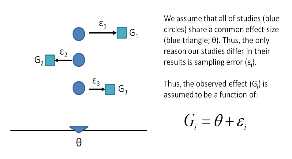
11.5.1 Fixed Effects Model
Under the fixed effect model we assume that there is one true effect size which is shared by all the included studies. It follows that the combined effect (global estimate) is our estimate of this common effect size.
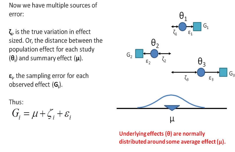
11.5.2 Random Effects Model
- Under the random effects model we allow that the true effect could vary from study to study. E.g. the effect size might be a little higher if the patients are older; in rats vs. mice; if the study used a slightly more intensive or longer variant of the intervention etc.
- The studies included in the meta-analysis are assumed to be a random sample of the relevant distribution of effects, and the combined effect estimates the mean effect in this distribution.
11.6 Step 3. Investigate heterogeneity
The third step is to investigate potential sources of heterogeneity (pre-specified in your protocol). Heterogeneity is the variability between groups of studies caused by differences in:
- study samples (e.g. species, sex)
- interventions of outcomes (e.g. dose, outcome measure type)
- methodology (e.g. design, quality)
Chi-squared \(\chi^2\) (or Chi2) assess whether observed differences in results are compatible with chance alone. I2 describes the percentage of variability in effect estimates that is due to heterogeneity rather than sampling error or chance along.
You can investigate heterogeneity using:
- Sub-group analysis. Read more about sub-group analysis here.
- Meta-regression model. Read more about meta-regression here.
11.7 Step 4. Reporting biases
Publication Bias occurs when the results of published and unpublished studies differ systematically. Unfortunately, neutral and negative studies take longer to be published, remain unpublished, are less likely to be identified in systematic review, and this can lead to an overstatement of efficacy in meta-analysis.
There are also other biases that may effect your systematic review including, selective outcome reporting and selective analysis reporting.
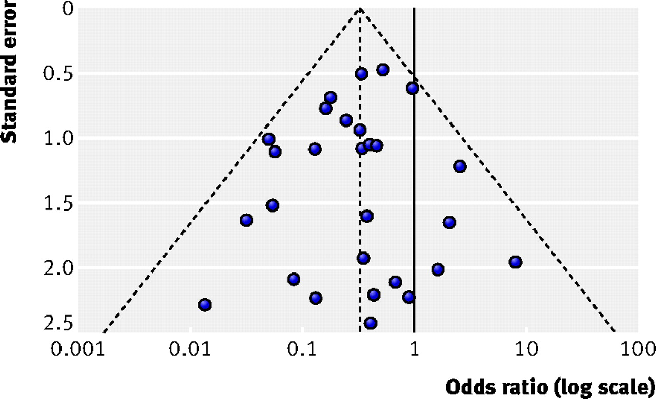
We can test for potential publication bias in our data plotting our data on a funnel plot. The outer dashed lines indicate the triangular region within which 95% of studies are expected to lie, in the absence of both biases and heterogeneity. The solid vertical line refers to the line of no effect. Image from Sterne et al., 2011
If you do observe asymmetry in your funnel plot, there may be a number of sources:
Reporting Biases
- Publication bias
- Selective outcome reporting
- Selective analysis reporting
Poor methodological quality (leading to inflated effects in smaller studies)
- Poor methodological design
- Inadequate analysis
- Fraud
True heterogeneity: Effect size differs according to study size due to e.g. differences in the intensity of interventions, or in underlying risk between studies with different sizes.
Artefacts: Sampling variation can lead to an association between the intervention effect and its standard error.
Chance: Asymmetry may occur by change - motivating the use of statistical asymmetry tests.
11.8 Step 5. Interpret the results
The forest plot or timber plot is the main graphical output or representation from a meta-analysis.
Reading and understanding these plots will allow you to understand the findings from a meta-analysis. Meta-analyses of animal studies tend to include many studies with small sample sizes. Therefore, it is common to see preclinical meta-analyses graphically represented with a timber plot, a slight variation on the forest plot.
Here is an example of a timber plot. In this meta-analysis the research question was: What is the effect of antidepressants compared vehicle or no treatment on infarct volume in animal models of ischaemic stroke? McCann et al., 2014
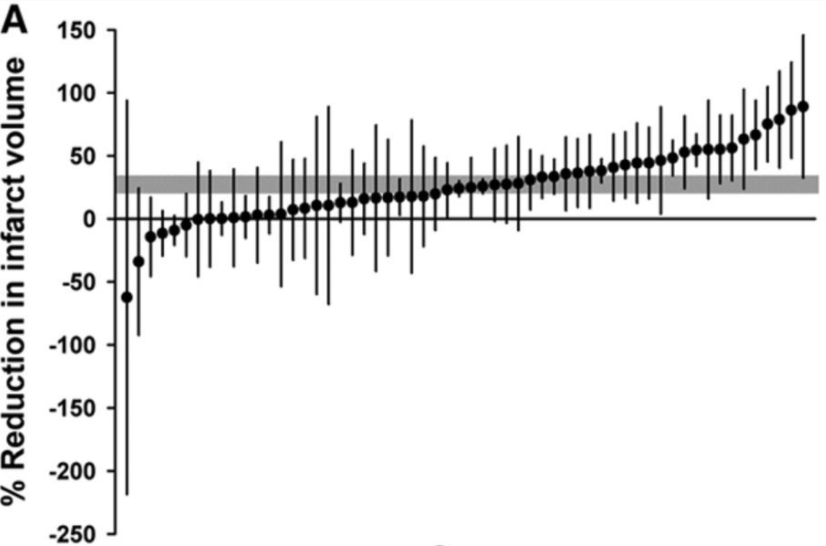
Outcome: A meta-analysis is conducted on a single outcome of interest at a time. The outcome of interest in this meta-analysis is Reduction in Infarct Volume, as displayed on the y-axis label.
Individual Study Effects: In this meta-analysis there were 58 experiments included. Each black dot represents the effect size reported in a single experiment, the difference in outcome between the mean and the control group. Each black dot has thin black lines above and below the effect size, these represent the errors bars associated with the effect size reported. Individual study effect sizes are displayed in order of smallest to largest to highlight variation or heterogeneity in the literature.
Pooled Effect: Here, the gray bar behind the black dots represents the combined or pooled effect size across all included experiments and its confidence intervals. In this example, the effect size is 27.3% (95% CI, 20.7%–33.8%).
Clinical Forest Plots: A step-by-step guide to interpreting a forest plot from a typical clinical meta-analysis is available here.
Website by A Bannach-Brown on behalf of CAMARADES & CAMARADES Berlin
CAMARADES.Berlin@charite.de

This work is licensed under a Creative Commons Attribution 4.0 International License.